Elasticsearch: Adventures in scaling a multitenant platform

Running Elasticsearch at scale can be challenging by itself. When adding multitenancy to the equation it can be hard to know what direction to take. At BigCommerce we use Elasticsearch for all the search features on our clients storefronts. As a SaaS provider we host all sorts of different customers with different requirements for their storefronts. Some stores may only have a few products (10-100), while some stores have more than 3 million (such as stores dedicated to auto parts). Stores also have different traffic patterns. A small site may get many hits per second, while a larger store might get only a few 100 hits every day.
The navigation of some stores on our platform use faceted search as a means of navigating the entire product catalog, resulting hits to the Elasticsearch cluster for each page load of the storefront. Search bots indexing these stores can produce a large number of requests in a relatively short time frame.
While our storefront searches would push us towards being more read heavy, some of the workflows our customers use can involve many updates to their products on a daily basis, sometimes this can mean re-submitting their entire product catalogue, so we need to be making various concessions towards write speed too. Once a product is updated we should have access to content in search pretty quickly too (more on this here).
Elasticsearch for Newbies
If you’re reasonably new to Elasticsearch you should familiarise yourself with some of the basic concepts so you can keep pace with the rest of this article:
- Node types: Data, Client
- Indexes
- Shards and Replicas
- Documents
- Fields
In simplistic terms, each piece of data in Elasticsearch is represented as a document, which is made up of fields. In traditional RDBMS terminology it might help you to consider a document as a table row and a field as a table column (although this is an overly simplistic view as documents can have different fields, unlike the fixed set of columns in a database table).
Each document is stored in an index. This index is stored in a predefined number of shards which are distributed over the data nodes. These shards are Apache Lucene indexes that store the documents with inverted indexes. Usually a shard has a replica which sits on another server, this helps ensure data is still available when the node with the primary shard is not available.
Search queries are sent by clients to the client nodes, these are routed to the correct index / shard and the query is sent to the required data nodes. This includes sending the query to data nodes containing the replica. The client node collects the responses, combines them, sorts the result and returns it to the client.
Issues with Previous Platform
Our previous production platform assigned each store to a single shard, in a single index. With limited information available at the time of implementation (early 2014) and without a reasonably defined set of product requirements, the hypothesis was that it would be faster for Elasticsearch to only have to query a single shard rather than broadcasting the query over the entire cluster of up to 60+ shards (120+ with replicas). To an extent this is true, but practically however, this does produce many issues:
- Stores with big catalogs could create shards upto 150GB
- elastic.co recommends shards be less than 50GB
- Unbalanced shards, data is not distributed evenly over all shards
- Massive shards take a significant amount of time to relocate when the index is re-sharded
- Massive shards cause heap stress resulting in heavy Garbage Collection and stop the world events
- Routed index causes nodes with big shards to get "hot"
- Often seen during traffic bursts and site crawling
- Causes poor responses times for other stores on shards on those nodes
- Causes GC pauses on nodes
At the time, our production environment (running an antique 1.7.3 release) was using 23 (mostly unutilised) data nodes to cope with our daily average peaks. When we got a traffic spike or a site being crawled it negatively affected response times and caused searches to be queued or worse, rejected. To scale the cluster we’d just add more data nodes, but that would only buy us a small amount of time, didn’t smooth out the hotspots or solve the problem of the garbage collection pauses.
Additionally, a single large index coupled with large shards required substantial amounts of memory to process aggregations (aka facets, product filters). This only got worse as we provisioned more stores. This had resulted in faceted search queries failing entirely due to circuit breakers being triggered. As a work around for the poor performance we had to temporarily disable the product counts on some of the filters which were particularly memory intensive:
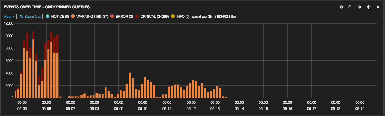
The above graph shows the number of HTTP 500 errors for /catalog requests up until we disabled the product counts
This also demonstrated how cumulative effects can have a substantial impact on many areas of a complex system. General search performance, indexing speed and garbage collection were improved:
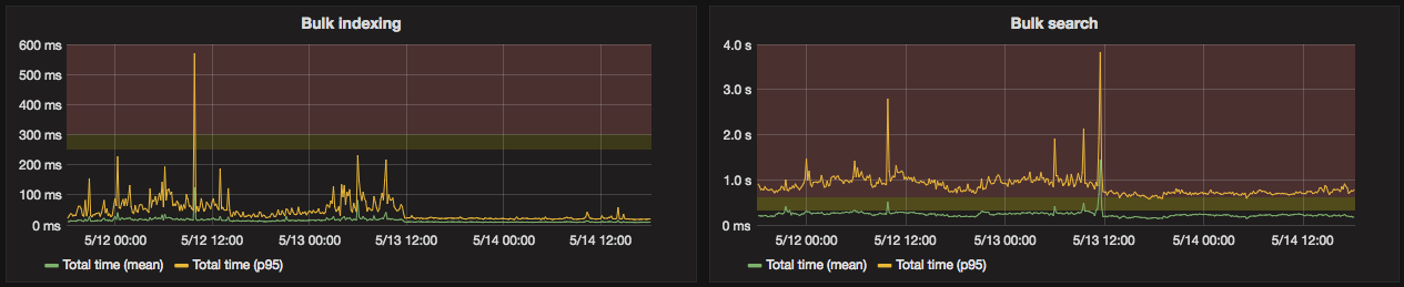
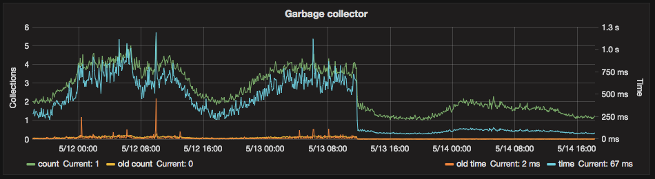
While these response time improvements are great, reductions in functionality do not resolve the underlying issues and provide a poor experience for our merchants and their customers. These were simply stop gap measures to keep things running a bit more smoothly.
In an Elasticsearch outage in 2015, we tried to convert our 160 shard single index from routed queries to non-routed queries. That is to say, we created a new index that would store documents for all store across all the shards within the index. The idea here was that we would share the load better, reducing shard sizes and reducing garbage collection time and frequency. Sadly, this failed spectacularly with massive garbage collection stalls taking out the entire platform. After this, we decided to go back to the drawing board.
Back to the Drawing Board
All our attempts to tame the production platform had failed. This was going to take more than a quick config tweak that we found at the back of some dark and dank corner of stack exchange… This was going to take some real planning, good quality engineering and most importantly, time. We needed to take a big step back and figure out what we needed from our platform. This led us to the following requirements
Requirements for new Platform:
- Must be scalable to allow faceted search for all stores
- Should limit shard sizes to <50GB (As recommended by elastic.co)
- Should limit JVM heap size to around 16GB (Maximum ~31GB) (to reduce GC times)
- Must be able to meet and exceed current and historical load from current platform
- Should stick to Elasticsearch default configurations as much as possible, the fewer tweaks the better.
- Improved visualization into the entire cluster.
- Engineering access to cluster visualisation tools.
- Use the latest version of Elasticsearch (2.3.x) which brings substantial performance improvements (especially regarding parent/child queries)
Yowsers… based on our experience with Elasticsearch to date, they are some pretty ambitious goals.
"But wait..." I hear you say, “... surely building a multitenant cluster designed for scaling can’t be that hard?” Well my friend, in the wise words of Elasticsearch support engineers when asked how to scale: “It depends”. The profile of your data, how you index it and how you search it are all highly variable. No one solution fits all. The only way to scale for your use case is to go and test it and find what works.
So with this in mind, we did our research, watched a bunch of videos, read reams of documentation, and did much pondering. We knew that routing a store to an individual shard was bad, but spreading all stores documents across all shards was also bad. We needed a middle ground where we could get the benefits of distributed computing, but not so much that we have to search across 120 shards to find the data for one store. Thankfully, we ran across something seemingly perfect for our use case: Shard Allocation Filtering
Using shard allocation filtering, we can create multiple indexes and assign their shards to particular nodes, essentially creating small clusters within the overall larger cluster. A store would then be assigned to a specific index. This also has the benefit of separation of concerns and gives us a lot more control back. If a store is overly impacting others in the index then we can now move it to a lesser utilised index, much like we can do with our database clusters. Additionally, we control the exact number of shards an index uses as we move forward, giving us the flexibility to be able to change and improve as we build out.
We threw together a design proposal and fired it across to the wizards at elastic.co to give it a once over. After reviewing the documentation we provided, elastic.co informed us that Shard Allocation Filtering was initially designed more for utilising lower power (and therefore cost) hardware for less frequently accessed indexes (a.k.a old Logstash Indexes). They encouraged us to test the performance of our proposed usage before proceeding. So that’s what we did!
Adventures in Elasticsearch Performance Testing
Now, This section might get a bit glossed over… but there was a huge effort involved to get something setup that was at least a micro-analogue of our production infrastructure.
Based on the design proposal (using shard allocation filtering) we built out the following in AWS for testing:
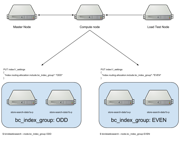
We used a tag of bc_index_group to allow us to allocate our indexes to specific nodes.
This was built separately from our existing infrastructure and services as we didn't want to affect anything in production. We also wanted a clean-room environment and we didn't use any of our current configurations or puppet manifests… this is pure ES, straight from the package.
We only have a single "compute" (client) node, and 4 data nodes. We added a master node as it’s not only best practice to separate it out but it’s a great place to put cluster management tools such as Marvel and Kopf.
To give us a rough match with hardware we are currently running in production, all machines were the following specs:
| Data | Client | Loadtest | |
|---|---|---|---|
| AWS Machine Type | c4.4xlarge | c4.2xlarge | c4.4xlarge |
| vCPUs | 16 | 8 | 16 |
| Memory | 30 GB | 15 GB | 30 GB |
| Storage | 4x 100GB EBS in RAID1 @ 1920 IOPS | 8GB EBS | 8GB EBS |
Populating the instance with data
We extracted a list of all our stores that had the faceted search feature available on their store plan (though not necessarily using it). At the time this came out at around 7000 stores. We re-indexed a copy of their publicly facing catalog data into the test lab. This equated to 100 million documents (31m parent docs with 59m nested docs) and about 58GB of disk storage. We wanted to use the copy of the real production data here so that we could get a reasonably accurate mix of products, facets, document sizes and catalog sizes. It would be a challenge to reproduce this diversity with an algorithm to produce similar data.
Now we had a decent subset of data on a reasonable analogue, what to do about loading it with requests. We keep the Elasticsearch query logs in logstash, so using the scroll API to query the underlying ES cluster, we extracted 24 hours worth of queries for the specific set of stores, which came out to around 9M queries.
To allow us to split up the different type of queries, the search query file was in the format of: TIMESTAMP.MS|SEARCH_TYPE|JSON_QUERY
Example entry:
1451880953.249|product|{"sort": [{"_score": {"order": "desc", "ignore_unmapped": true}}], "query": {"filtered": {"filter": {"bool": {"must": [{"term": {"store_id": 123456}}, {"bool": {"_cache": true, "should": [{"term": {"_cache": false, "inventory_tracking": "none"}}, {"range": {"_cache": false, "inventory_level": {"gte": 1}}}]}}, {"term": {"is_visible": true}}]}}, "query": {"bool": {"should": [{"simple_query_string": {"query": "Google Nexus 5x", "fields": ["name^2", "name.partial", "description", "sku^3", "sku.partial", "keywords^2", "keywords.partial", "brand_name^2"]}}, {"prefix": {"sku": {"boost": 1, "value": "Google Nexus 5x"}}}, {"prefix": {"keywords": {"boost": 1, "value": "Google Nexus 5x"}}}]}}}}, "_source": ["store_id"], "from": 0, "size": 6}
Elasticsearch log replay
We needed a tool that would let us easily produce load patterns against our AWS lab infrastructure by submitting multiple JSON query payloads over HTTP. This required a tool that was able to alternate the index easily too. The logical choice for us was JMeter.
We used two different test plans. The first would split queries between aggregated search and regular search queries, the second test script split queries based on odd and even numbered store ids.
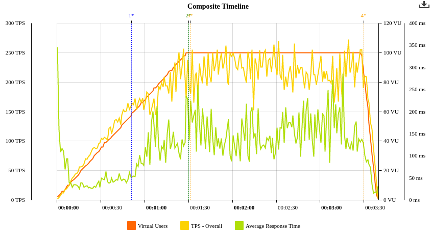
We configured a ramp-up stage and a constant stage with tests totalling 3 minutes of run time. This would ensure that we didn’t flood the cluster immediately and skew the results (due to cold caches).
Here you can see the ramp up stage and the constant stage, this allowed us to see clearly where the system was overloaded. We peak at 100 concurrent Virtual Users. Each virtual user would run in a constant loop to send a Regular query, then sleep for 300ms, then send an Aggregated searcg query before starting the loop again.
Of the 9 million queries in the list, this test plan only ended up using about 48,000 queries in the 3 minute test.
To analyse the results we used BlazeMeter Sense. A JMeter plugin allows the results to automatically be uploaded during the test run allowing us to watch the tests in real-time as they were running. Once complete, BlazeMeter would analyse the results and give us great statistics and graphs regarding our tests. You can see one of our publicly shared results here: http://sense.blazemeter.com/examples/517543/
We've dumped a copy of the test plan's we used in a couple of gists:
For the impatient here is an awesome graph:
Systems monitoring
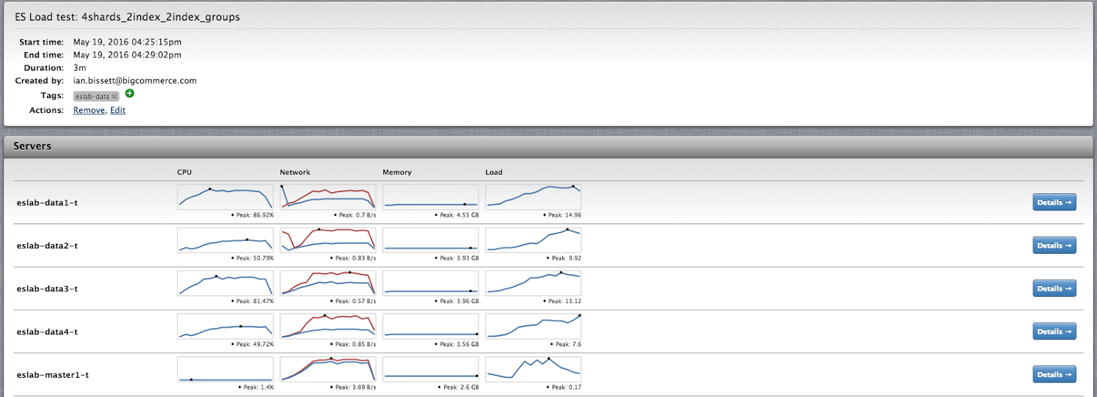
To monitor the systems during testing we used quick and easy cloud tools so we could keep moving quickly. We are outside of our current platform, so feeding metrics into graphite could have taken quite some time to get going.
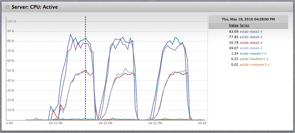
As we already had a CopperEgg account we used it to monitor server health. This was cool as we could set annotations using the API to quickly see on the graphs which test was running when and the resuslts that test had on the hardware.
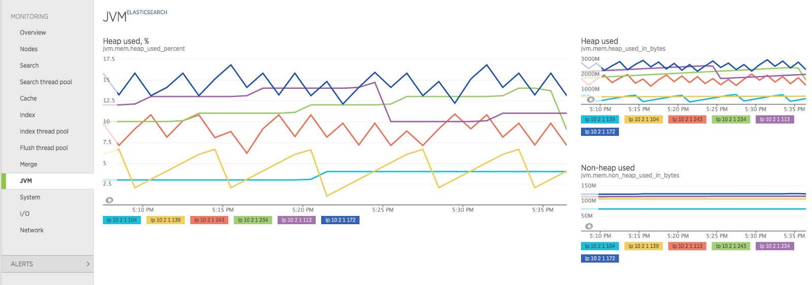
To get metrics on Elasticsearch we used a mix of Marvel, Kopf and a plugin for NewRelic that gave us access to statistics on ES and the JVM:
Here’s an example snapshot of some of the many different sharding/index patterns we produced as we commenced testing.
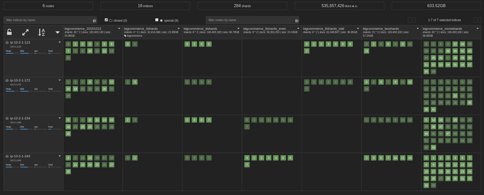
Notice that the bigcommerce_8shards_odd and bigcommerce_8shards_even are on totally separate hosts. This is the shard allocation filtering at work.
Elasticsearch doesn't allow an index to be copied, so testing a new configuration means creating the index from scratch and freshly indexing the documents into it. Fortunately, Elasticsearch recently implemented a handy reindex API to scan through all the data from a source and index it into a destination. This process would still take around 3-4 hours however due to the fairly large number of documents we are dealing with.
Setting the Benchmark
The original plan was to either benchmark from the existing production cluster or to use our staging platform. However, not wanting to impact an already fragile system or to disrupt staging, we instead opted to set a benchmark on the new lab nodes with base Elasticsearch settings and a single non-routed (ie. the default behaviour) index of 30 shards. This would give us a baseline to improve upon.
Down the Rabbit Hole
We didn't quite find a rabbit in a waistcoat… but we were in a topsy-turvy world where very little made sense.
Before we ran each experiment (and repeated it at least 3 times for data consistency, just like real scientists!) we would discuss what we expected the outcome to be, and almost every time Elasticsearch gave us the metaphorical finger. Each test was based around a simple hypothesis.
Hypothesis 1: As shard size increases, so should response time
We know that the larger the shard, the more content we need to scan through to find what we want. We also know that as we page a large shard through the JVM and lucene we need to use more heap, which is more likely to cause a garbage collection. So, as we decrease the number of shards, so should the size of the shards increase.
Results:
| Number of shards (+1 mirrored replica) | Median Shard Size (approx) | Average Response Time | 95th Percentile Response Time |
|---|---|---|---|
| 60 | 1GB | 741 ms | 1266 ms |
| 30 (benchmark) | 2GB | 518 ms | 1007 ms |
| 15 | 4GB | 304 ms | 695 ms |
| 8 | 8GB | 223 ms | 720 ms |
| 4 | 17GB | 134 ms | 600 ms |
Analysis:
As we decrease the number of shards, the shard sizes do increase, however, the opposite of what we expected happens. Having fewer shards increases the performance, seemingly regardless of the number of shards. We stopped at 4 shards as we do not intend to run with less that 4 shards in production.
What we think is happening here is that we do not have enough data to fully stress the JVM heap and cause the same kind of garbage collection we have been seeing on our production cluster.
It does show us however that reducing the number of shards reduces response time. We repeated this test and reduced the the heap size to 8GB to see if we could cause the heap stress we know and love despise… but alas, we could not reproduce it.
Hypothesis 2: Splitting a single index into 2 indexes with the same number of shards should make very little difference
By splitting our single index into separate indexes (but with the same number of total shards) should have little to no discernible overhead to the search process. That is to say if we split our single 15 shard index into two 8 shard indexes, we should get roughly (or even slightly worse as we have 1 more shard) the same performance.
For this test we split out the data from our odd numbered stores into one index, and the even numbered ones into a different index. We then updated our JMeter tests to query the different indexes.
Results:
| Original Number of shards: | 8 | 15 |
|---|---|---|
| Shards in each dual index: | 4 | 8 |
| Original Response Time (average): | 223ms | 304ms |
| Original Response Time (95th Percentile): | 720ms | 695ms |
| Dual index Response Time (average): | 48ms | 101ms |
| Dual index Response Time (95th Percentile) | 265ms | 200ms |
| Response Time Delta (average): | -175ms | -203ms |
| Response Time Delta (95th Percentile): | -455ms | -495ms |
Analysis:
Initial Thoughts: Sweet Zombie Jeebus?! What did we just do?! We just improved our average response times by over 400%, and our 95th Percentile improved by over 300%
Further more CPU consumption was reduced for the duration of the test and there was less garbage collection usage.
The question that plagued me for far too long was a very simple one: WHY? Why the frack did this make such an epic difference to the processing times. After sleeping on the problem it finally sank in.
To understand the problem fully, I had to draw a diagram that shows how a query hits shards in various scenarios:
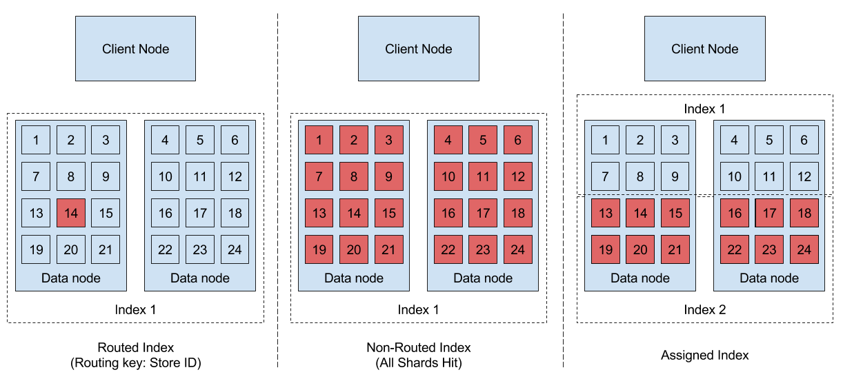
The red boxes are the shards that are hit during the query (for those reading on a black and white print out, the red boxes are the ones next to the blue ones).
When we are using a routed index, only a single shard is queried per store. When we are using a single index for all stores then every query hits ALL the shards. That is to say, Elasticsearch needs to execute 15 separate queries and return the relevant data to the client node. The response is returned only when all shards have completed their search.
With the "assigned index" scenario, each index has only half the data in half of the number of shards. So now to find the documents for any given store, we only need to query 8 shards so we only have to wait for those 8 shards to be searched. In this way, we’re not only getting the performance boost that we saw from Hypothesis 1 when moving from 15 to 8 shards, but we still have the benefit of a smaller shard size of a 15 shard index. It’s the best of both worlds. Going from 2x8 to 2x4 boosted performance even further.
In our actual production environment things are even more complicated. Multiple threads, multiple hosts and multiple indexes exagerate this performance gain even further.
Hypothesis 3: Splitting the indexes on to separate hosts will not add considerable overhead
The idea here is that if we can separate out an index onto it’s own set of hosts then we can separate out our areas of concern. That is to say that if one index is heavily loaded, then it won’t impact queries to another index as it’s hosted on different hardware.
To complete this test, we used shard allocation filtering to create index groups and put our odd numbered stores onto two data nodes and our even numbered stores onto two other nodes.
Results:
| 8 Shards per Index | 4 Shards per Index | |||
|---|---|---|---|---|
| Odd | Even | Odd | Even | |
| Distribution of data | 61% | 39% | 61% | 39% |
| Distribution of queries | 50% | 50% | 50% | 50% |
| Dual Index Response Time (Average) | 104 ms | 97 ms | 60 ms | 34 ms |
| Response Time with Index Groups (Average) | 225 ms | 82 ms | 108 ms | 41 ms |
| Response Time Delta (Average) | +121 ms | -15 ms | +48 ms | +7 ms |
(95th percentile data is not available for the odd vs even queries)
Analysis:
These results indicate that the "even" index responded more quickly than the larger “odd” index. On the backend we saw a notably more CPU load on the servers managing the “odd” index.
Based purely on the "even" index, we are comfortable saying that the index groups do not add additional overhead to the query times. We can also comfortably say that the index groups are an effective way of shielding parts of the infrastructure during high load scenarios.
Practically however, we’ll likely host several indexes on each host, much like the setup in Hypothesis 2. This will get better utilisation of hardware resources. This is mostly due to not wanting to overallocate memory to the JVM. Heap sizes are effectively limited to ~31GB and experience has shown as that even this is too large. A heap of this size can take a significant amount of time to perform garbage collection and can lead to stop-the-world scenarios. On occasion this has caused a node to be completely unresponsive, resulting in it getting ejected from the cluster, forcing shard re-allocation and producing cascading issues across the rest of the data nodes in the cluster. It’ll be more efficient to have smaller sets of data hosted into smaller heaps. GC’s may happen more frequently, but they’ll process more quickly.
The proof is in the pudding
We had been limping along with a poor performing cluster for so long that we were blinded by our original assumptions… we were stuck in the "one more tweak will fix it" mode. It was a big leap for us to decide to stop working on trying to fix the old platform and instead spend a few weeks on testing a totally new cluster. Without taking things all the way back, it was difficult to drop our assumptions, and in the end, all the time and effort has proved to be worth it.
We decided to build a new cluster using the index groups that are built around shard allocation filtering to segregate load across nodes in the cluster. We now have many indexes within each index group but each index has a very small number of shards.
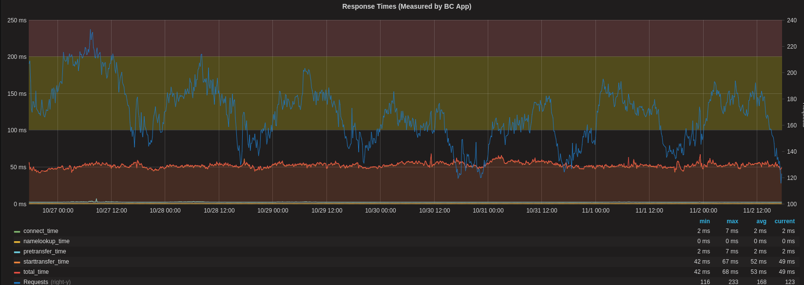
We built out the new cluster earlier this year and migrated stores to the new cluster progressively. Here’s how our response time looked after we had migrated around 50% of stores:
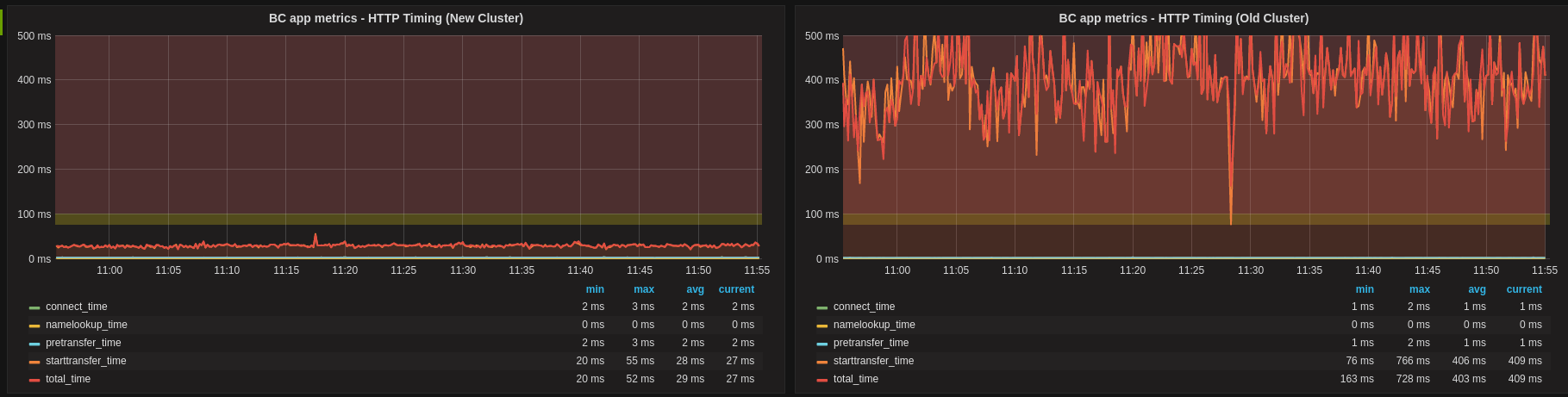
These days the response time on our platform looks more like this:
And here’s what happens now when we have a spike of requests from GoogleBot:
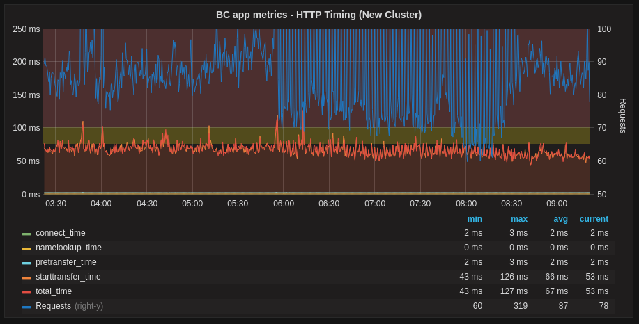
As a result of this work we managed to reduce the average response time of our search requests from an arguably awful ~700ms peak down to a much more manageable ~25ms per request.
Even more excitingly, we’ve taken our 95th percentile down from a rather embarrassing average of over 4 seconds to a much more manageable ~50ms.
This has enabled us to open more search features to more of our stores, enabling our clients to sell more!